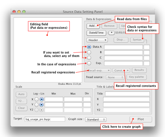
1. Preparation

The following window is Source Data Setting Panel. What you have to do at first when you create a graph with ByeGraph is to set necessary items, which are Data or Expressions, graph labels and scales, in this panel for creating a graph.

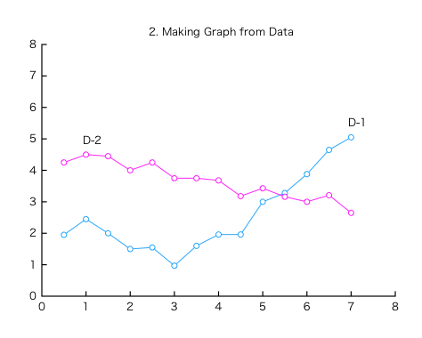
This panel is used for all of documents opening at present, and displays settings for the most front document. Graph output is always aimed at the most front document.

2. Making Graph from Data

To set data, you can specify particular data files from the "Add…" button, or can directly enter them into the editing field. (You can set totally up to three sets of data from Data A to Data C.)

Basically, the first column data must be x ones. And y data need to be set from the second column as many as you want. (According to your graph's type, you can change the position of x data, or need not put any x data.) Each of data in a line needs to be separated by space, tab or comma.

%label "D-1" "D-2"
%symbol b ! Plotting with Symbol-Line combination
0.5   1.95   4.25
1.0   2.45   4.50
1.5   2.00   4.45
2.0   1.50   4.00
2.5   1.55   4.25
3.0   0.97   3.75
3.5   1.60   3.75
        :
        :

The two lines starting with "%" before data lines are called "Header" and are used to specify various settings for creating a graph. The %label header is for specifying "Data labels". The %symbol header is for specifying the combination of symbol and line. Except for these, there are many kinds of headers, such as headers for settings for axes or scales, headers for specifying a graph type, and so on. Many of headers can be omitted because the settings of those can be specified after that manually. But according to the type of a graph, there are some headers which cannot be omitted. And regarding scale settings, If you do not use the related headers, proper scale values are set taking account of the maximum values of data.

After you check the syntax of the data, click the Plot button to create a desired graph.

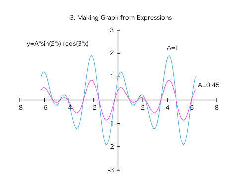
3. Making Graph from Expressions

Choose the Expression section and enter expressions into the Expression field. (Or you can recall expressions that have been used before from the "Recall Exp." pop-up menu.)

%label "A=1" "A=0.45"
%axislabel title "y=A*sin(2*x)+cos(3*x)"
x=<-2*pi:2*pi:0.02*pi>@
sa=2*x@
ca=3*x@
A={1,0.45}@
y=A*(sin(sa)+cos(ca))

You can put headers also prior to expressions. There are two types of headers that can be used in expressions: common headers with data and dedicated headers for expressions. The %axislabel header can be used also in data and is for specifying a title or axis labels for a graph. (In this example, it specifies a title.)

Each of expressions has to be separated by @, and "y=" has to be put at the beginning of the last expression. You can specify the range of the loop variable with x=<::>. Its arguments are the initial value, the maximum value and the step value from the left. And you can specify parameters with "Variable" ={,,,}. Y data are outputted up to the same number as parameters. You are allowed to put parameters in multiple places.

After you check the syntax of the expressions, click the Plot button to create a desired graph.

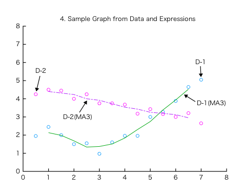
4. Combination of Data and Expressions

The examples (2) and (3) showed how each of data and expressions is solely transformed into a graph. This example will show how a combination of data and expressions is transformed into a graph.

Having a file-reading-function in expressions enables data to be read from the outside of the expressions, and to be used for calculation. In this example, moving average will be calculated from the data which was used in the example (2), and the calculation results will be plotted over the original data. The following is the same as the data of the example (2) apart from the parameter of the %symbol header.

%label "D-1" "D-2"
%symbol s ! Change the combination to Symbol only
0.5   1.95   4.25
1.0   2.45   4.50
1.5   2.00   4.45
2.0   1.50   4.00
2.5   1.55   4.25
3.0   0.97   3.75
3.5   1.60   3.75
        :
        :

There are two types of file-reading-functions, fread and fread2. The fread function reads data from the outside sequentially, on the other hand, the fread2 function reads at random. In this example, the fread2 function will be used, because a targeted data has to be read with front and back data of it at one time if you make your expressions do moving average. You need to choose a source data for the file-reading-function from Data A, B, C and an external file by using the "fread source" pop-up menu. (If you use an external file, you need to specify a path to the external file with the %external header.)

%label "D-1(MA3)" "D-2(MA3)"
%symbol l ! Plotting with Line only
%linetype 2 3
n=<1:#FREADMAX-2:1>@
x=fread2(n,0)@
w={1,2}@
z=sum(fread2(n+k,w),k=-1:1)@
y=z/3

#FREADMAX is the constant which stands for the line depth of a source data for file-reading-functions. By using this constant, you can continue to use your expressions without modification even if the source data is changed and the depth of it differs from the previous.

After you check the syntax of the data and the expressions, click the Plot button to create a desired graph. (On the graph below, some line objects (arrows) are added after graph creation.)